mirror of
https://github.com/jkriege2/JKQtPlotter.git
synced 2024-12-25 18:11:38 +08:00
252 lines
15 KiB
Markdown
252 lines
15 KiB
Markdown
# Tutorial (JKQTPDatastore): Advanced 1-Dimensional Statistics with JKQTPDatastore {#JKQTPlotterBasicJKQTPDatastoreStatistics}
|
|
|
|
[JKQTPlotterBasicJKQTPDatastore]: @ref JKQTPlotterBasicJKQTPDatastore "Basic Usage of JKQTPDatastore"
|
|
[JKQTPlotterBasicJKQTPDatastoreIterators]: @ref JKQTPlotterBasicJKQTPDatastoreIterators "Iterator-Based usage of JKQTPDatastore"
|
|
[JKQTPlotterBasicJKQTPDatastoreStatistics]: @ref JKQTPlotterBasicJKQTPDatastoreStatistics "Advanced 1-Dimensional Statistics with JKQTPDatastore"
|
|
[JKQTPlotterBasicJKQTPDatastoreRegression]: @ref JKQTPlotterBasicJKQTPDatastoreRegression "Regression Analysis (with the Statistics Library)"
|
|
[JKQTPlotterBasicJKQTPDatastoreStatisticsGroupedStat]: @ref JKQTPlotterBasicJKQTPDatastoreStatisticsGroupedStat "1-Dimensional Group Statistics with JKQTPDatastore"
|
|
[JKQTPlotterBasicJKQTPDatastoreStatistics2D]: @ref JKQTPlotterBasicJKQTPDatastoreStatistics2D "Advanced 2-Dimensional Statistics with JKQTPDatastore"
|
|
[statisticslibrary]: @ref jkqtptools_math_statistics "JKQTPlotter Statistics Library"
|
|
|
|
This tutorial project (see `./examples/datastore_statistics/`) explains several advanced functions of JKQTPDatastore in combination with the [[statisticslibrary]] conatined in JKQTPlotter.
|
|
|
|
***Note*** that there are additional tutorial explaining other aspects of data mangement in JKQTPDatastore:
|
|
- [JKQTPlotterBasicJKQTPDatastore]
|
|
- [JKQTPlotterBasicJKQTPDatastoreIterators]
|
|
- [JKQTPlotterBasicJKQTPDatastoreStatistics]
|
|
- [JKQTPlotterBasicJKQTPDatastoreRegression]
|
|
- [JKQTPlotterBasicJKQTPDatastoreStatisticsGroupedStat]
|
|
- [JKQTPlotterBasicJKQTPDatastoreStatistics2D]
|
|
|
|
[TOC]
|
|
|
|
The source code of the main application can be found in [`datastore_statistics.cpp`](https://github.com/jkriege2/JKQtPlotter/tree/master/examples/datastore_statistics/datastore_statistics.cpp).
|
|
This tutorial cites only parts of this code to demonstrate different ways of working with data for the graphs.
|
|
|
|
# Generating different sets of random numbers
|
|
|
|
The code segments below will fill four instances of JKQTPlotter with different statistical plots. All these plots are based on three sets of random numbers generated as shown here:
|
|
```.cpp
|
|
size_t randomdatacol1=datastore1->addColumn("random data 1");
|
|
size_t randomdatacol2=datastore1->addColumn("random data 2");
|
|
size_t randomdatacol3=datastore1->addColumn("random data 3");
|
|
std::random_device rd; // random number generators:
|
|
std::mt19937 gen{rd()};
|
|
std::uniform_int_distribution<> ddecide(0,1);
|
|
std::normal_distribution<> d1{0,1};
|
|
std::normal_distribution<> d2{6,1.2};
|
|
for (size_t i=0; i<150; i++) {
|
|
double v=0;
|
|
const int decide=ddecide(gen);
|
|
if (decide==0) v=d1(gen);
|
|
else v=d2(gen);
|
|
datastore1->appendToColumn(randomdatacol1, v);
|
|
if (decide==0) datastore1->appendToColumn(randomdatacol2, v);
|
|
else datastore1->appendToColumn(randomdatacol3, v);
|
|
}
|
|
```
|
|
|
|
The column `randomdatacol1` will contain 150 random numbers. Each one is drawn either from a normal dirstribution N(0,1) (`d1`) or N(6,1.2) (`d2`). the decision, which of the two to use is based on the result of a third random distribution ddecide, which only returns 0 or 1. The two columns `randomdatacol2` and `randomdatacol3` only collect the random numbers drawn from `d1` or `d2` respectively.
|
|
The three columns are generated empyt by calling `JKQTPDatastore::addColumn()` with only a name. Then the actual values are added by calling `JKQTPDatastore::appendToColumn()`.
|
|
|
|
|
|
# Basic Statistics
|
|
|
|
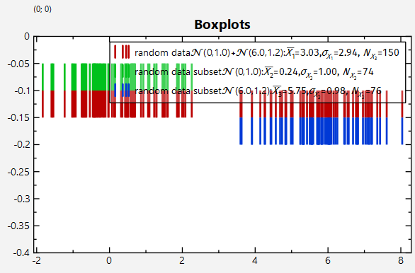
The three sets of random numbers from above can be visualized e.g. by a `JKQTPPeakStreamGraph` graph with code as follows:
|
|
```.cpp
|
|
JKQTPPeakStreamGraph* gData1;
|
|
plot1box->addGraph(gData1=new JKQTPPeakStreamGraph(plot1box));
|
|
gData1->setDataColumn(randomdatacol1);
|
|
gData1->setBaseline(-0.1);
|
|
gData1->setPeakHeight(-0.05);
|
|
gData1->setDrawBaseline(false);
|
|
```
|
|
|
|
This (if repeated for all three columns) results in a plot like this:
|
|
|
|
|
|
|
|
Based on the raw data we can now use JKQTPlotter's [statisticslibrary] to calculate some basic properties, like the average (`jkqtpstatAverage()`) or the standard deviation (`jkqtpstatStdDev()`):
|
|
|
|
```.cpp
|
|
size_t N=0;
|
|
double mean=jkqtpstatAverage(datastore1->begin(randomdatacol1), datastore1->end(randomdatacol1), &N);
|
|
double std=jkqtpstatStdDev(datastore1->begin(randomdatacol1), datastore1->end(randomdatacol1));
|
|
```
|
|
|
|
Both statistics functions (the same as all statistics functions in the library) use an iterator-based interface, comparable to the interface of the algorithms in the C++ standard template library. To this end, the class `JKQTPDatastore` provides an iterator interface to its columns, using the functions `JKQTPDatastore::begin()` and `JKQTPDatastore::end()`. Both functions simply receive the column ID as parameter and exist in a const and a mutable variant. the latter allows to also edit the data. In addition the function `JKQTPDatastore::backInserter()` returns a back-inserter iterator (like generated for STL containers with `std::back_inserter(container)`) that also allows to append to the column.
|
|
|
|
note that the iterator interface allows to use these functions with any container that provides such iterators (e.g. `std::vector<double>`, `std::list<int>`, `std::set<float>`, `QVector<double>`...).
|
|
|
|
The output of these functions is shown in the image above in the plot legend/key.
|
|
|
|
Of course, several other functions exist that calculate basic statistics from a column, e.g.:
|
|
- average/mean: `jkqtpstatAverage()`, `jkqtpstatWeightedAverage()`
|
|
- number of usable values in a range:`jkqtpstatCount()`
|
|
- minimum/maximum: `jkqtpstatMinMax()`, `jkqtpstatMin()`, `jkqtpstatMax()`
|
|
- sum: `jkqtpstatSum()`
|
|
- variance: `jkqtpstatVariance()`, `jkqtpstatWeightedVariance()`
|
|
- standard deviation: `jkqtpstatStdDev()`, `jkqtpstatWeightedStdDev()`
|
|
- skewnes`jkqtpstatSkewness()`
|
|
- statistical moments: `jkqtpstatCentralMoment()`, `jkqtpstatMoment()`
|
|
- correlation coefficients: `jkqtpstatCorrelationCoefficient()`
|
|
- median: `jkqtpstatMedian()`
|
|
- quantile: `jkqtpstatQuantile()`
|
|
- (N)MAD: `jkqtpstatMAD()`, `jkqtpstatNMAD()`
|
|
- 5-Number Summary (e.g. for boxplots): `jkqtpstat5NumberStatistics()`, `jkqtpstat5NumberStatisticsAndOutliers()`, `jkqtpstat5NumberStatisticsOfSortedVector()`, `jkqtpstat5NumberStatisticsAndOutliersOfSortedVector()`
|
|
|
|
All these functions use all values in the given range and convert each value to a `double`, using `jkqtp_todouble()`. The return values is always a dohble. Therefore you can use these functions to calculate statistics of ranges of any type that can be converted to `double`. Values that do not result in a valid `double`are not used in calculating the statistics. Therefore you can exclude values by setting them `JKQTP_DOUBLE_NAN` (i.e. "not a number").
|
|
|
|
|
|
# Boxplots
|
|
|
|
## Standard Boxplots
|
|
|
|
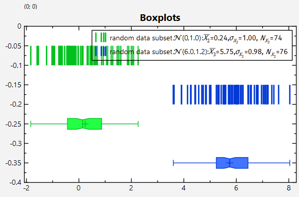
As mentioned above and shown in several other examples, JKQTPlotter supports [Boxplots](https://en.wikipedia.org/wiki/Box_plot) with the classes `JKQTPBoxplotHorizontalElement`, `JKQTPBoxplotVerticalElement`, as well as `JKQTPBoxplotHorizontal` and `JKQTPBoxplotVertical`. You can then use the 5-Number Summray functions from the [statisticslibrary] to calculate the data for such a boxplot (e.g. `jkqtpstat5NumberStatistics()`) and set it up by hand. Code would look roughly like this:
|
|
```.cpp
|
|
JKQTPStat5NumberStatistics stat=jkqtpstat5NumberStatistics(data.begin(), data.end(), 0.25, .5);
|
|
JKQTPBoxplotVerticalElement* res=new JKQTPBoxplotVerticalElement(plotter);
|
|
res->setMin(stat.minimum);
|
|
res->setMax(stat.maximum);
|
|
res->setMedian(stat.median);
|
|
res->setMean(jkqtpstatAverage(first, last));
|
|
res->setPercentile25(stat.quantile1);
|
|
res->setPercentile75(stat.quantile2);
|
|
res->setMedianConfidenceIntervalWidth(stat.IQRSignificanceEstimate());
|
|
res->setDrawMean(true);
|
|
res->setDrawNotch(true);
|
|
res->setDrawMedian(true);
|
|
res->setDrawMinMax(true);
|
|
res->setDrawBox(true);
|
|
res->setPos(boxposX);
|
|
plotter->addGraph(res);
|
|
```
|
|
|
|
In order to save you the work of writing out this code, the [statisticslibrary] provides "adaptors", such as `jkqtpstatAddVBoxplot()`, which basically implements the code above. Then drawing a boxplot is reduced to:
|
|
|
|
```.cpp
|
|
JKQTPBoxplotHorizontalElement* gBox2=jkqtpstatAddHBoxplot(plot1box->getPlotter(), datastore1->begin(randomdatacol2), datastore1->end(randomdatacol2), -0.25);
|
|
gBox2->setColor(gData2->getKeyLabelColor());
|
|
gBox2->setBoxWidthAbsolute(16);
|
|
```
|
|
|
|
Here `-0.25`indicates the location (on the y-axis) of the boxplot. and the plot is calculated for the data in the `JKQTPDatastore` column `randomdatacol2`.
|
|
|
|
|
|
|
|
## Boxplots with Outliers
|
|
|
|
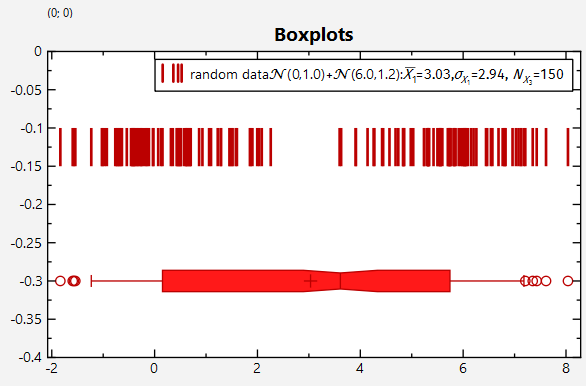
Usually the boxplot draws its whiskers at the minimum and maximum value of the dataset. But if your data contains a lot of outliers, it may make sense to draw them e.g. at the 3% and 97% quantiles and the draw the outliers as additional data points. This can also be done with `jkqtpstat5NumberStatistics()`, as you can specify the minimum and maximum quantile (default is 0 and 1, i.e. the true minimum and maximum) and the resulting object contains a vector with the outlier values. Then you could add them to the JKQTPDatastore and add a scatter plot that displays them. Also this task is sped up by an "adaptor". Simply call
|
|
|
|
```.cpp
|
|
std::pair<JKQTPBoxplotHorizontalElement*,JKQTPSingleColumnSymbolsGraph*> gBox1;
|
|
gBox1=jkqtpstatAddHBoxplotAndOutliers(plot1box->getPlotter(), datastore1->begin(randomdatacol1), datastore1->end(randomdatacol1), -0.3,
|
|
0.25, 0.75, // 1. and 3. Quartile for the boxplot box
|
|
0.03, 0.97 // Quantiles for the boxplot box whiskers' ends
|
|
);
|
|
```
|
|
|
|
As you can see this restuns the `JKQTPBoxplotHorizontalElement` and in addition a `JKQTPSingleColumnSymbolsGraph` for the display of the outliers. The result looks like this:
|
|
|
|
|
|
|
|
|
|
|
|
# Histograms
|
|
|
|
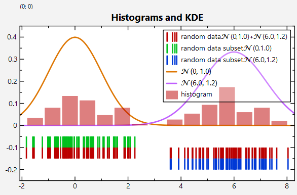
Calculating 1D-Histograms is supported by several functions from the [statisticslibrary], e.g. `jkqtpstatHistogram1DAutoranged()`. You can use the result to fill new columns in a `JKQTPDatastore`, which can then be used to draw the histogram (here wit 15 bins, spanning the full data range):
|
|
|
|
```.cpp
|
|
size_t histcolX=plotter->getDatastore()->addColumn(histogramcolumnBaseName+", bins");
|
|
size_t histcolY=plotter->getDatastore()->addColumn(histogramcolumnBaseName+", values");
|
|
jkqtpstatHistogram1DAutoranged(first, last, plotter->getDatastore()->backInserter(histcolX), plotter->getDatastore()->backInserter(histcolY), 15);
|
|
JKQTPBarVerticalGraph* resO=new JKQTPBarVerticalGraph(plotter);
|
|
resO->setXColumn(histcolX);
|
|
resO->setYColumn(histcolY);
|
|
resO->setTitle(histogramcolumnBaseName);
|
|
plotter->addGraph(resO);
|
|
```
|
|
|
|
Again there are "adaptors" which significanty reduce the amount of coude you have to type:
|
|
|
|
```.cpp
|
|
JKQTPBarVerticalGraph* hist1=jkqtpstatAddHHistogram1DAutoranged(plot1->getPlotter(), datastore1->begin(randomdatacol1), datastore1->end(randomdatacol1), 15);
|
|
```
|
|
|
|
The resulting plot looks like this (the distributions used to generate the random data are also shown as line plots!):
|
|
|
|
|
|
|
|
|
|
|
|
# Kernel Density Estimates (KDE)
|
|
|
|
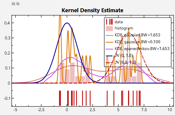
Especially when only few samples from a distribution are available, histograms are not good at representing the underlying data distribution. In such cases, [Kernel Density Estimates (KDE)](https://en.wikipedia.org/wiki/Kernel_density_estimation) can help, which are basically a smoothed variant of a histogram. The [statisticslibrary] supports calculating them via e.g. `jkqtpstatKDE1D()`:
|
|
|
|
```.cpp
|
|
size_t kdecolX=plotter->getDatastore()->addColumn(KDEcolumnBaseName+", bins");
|
|
size_t kdecolY=plotter->getDatastore()->addColumn(KDEcolumnBaseName+", values");
|
|
jkqtpstatKDE1D(first, last, -5.0,0.01,10.0, plotter->getDatastore()->backInserter(kdecolX), plotter->getDatastore()->backInserter(kdecolY), kernel, kdeBandwidth);
|
|
JKQTPXYLineGraph* resO=new JKQTPXYLineGraph(plotter);
|
|
resO->setXColumn(kdecolX);
|
|
resO->setYColumn(kdecolY);
|
|
resO->setTitle(KDEcolumnBaseName);
|
|
resO->setDrawLine(true);
|
|
resO->setSymbolType(JKQTPNoSymbol);
|
|
plotter->addGraph(resO);
|
|
```
|
|
|
|
The function accepts different kernel functions (any C++ functor `double f(double x)`) and provides a set of default kernels, e.g.
|
|
- `jkqtpstatKernel1DEpanechnikov()`
|
|
- `jkqtpstatKernel1DGaussian()`
|
|
- `jkqtpstatKernel1DUniform()`
|
|
- ...
|
|
|
|
The three parameters `-5.0, 0.01, 10.0` tell the function `jkqtpstatKDE1D()` to evaluate the KDE at positions between -5 and 10, in steps of 0.01.
|
|
|
|
Finally the bandwidth constrols the smoothing and the [statisticslibrary] provides a simple function to estimate it automatically from the data:
|
|
```.cpp
|
|
double kdeBandwidth=jkqtpstatEstimateKDEBandwidth(datastore1->begin(randomdatacol1subset), datastore1->end(randomdatacol1subset));
|
|
```
|
|
|
|
Again a shortcut "adaptor" simplifies this task:
|
|
|
|
```.cpp
|
|
JKQTPXYLineGraph* kde2=jkqtpstatAddHKDE1D(plot1kde->getPlotter(), datastore1->begin(randomdatacol1subset), datastore1->end(randomdatacol1subset),
|
|
// evaluate at locations between -5 and 10, in steps of 0.01 (equivalent to the line above, but without pre-calculating a vector)
|
|
-5.0,0.01,10.0,
|
|
// use a gaussian kernel
|
|
&jkqtpstatKernel1DEpanechnikov,
|
|
// estimate the bandwidth
|
|
kdeBandwidth);
|
|
```
|
|
|
|
Plots that result from such calls look like this:
|
|
|
|
|
|
|
|
|
|
# Cummulative Histograms and KDEs
|
|
|
|
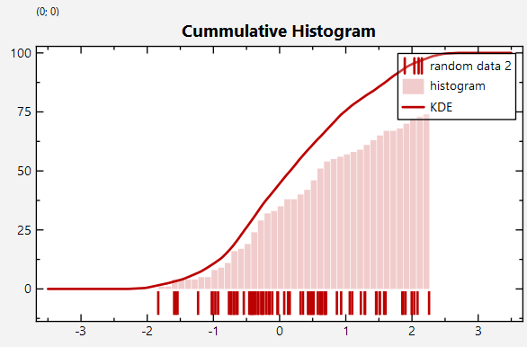
Both histograms and KDEs support a parameter `bool cummulative`, which allows to accumulate the data after calculation and drawing cummulative histograms/KDEs:
|
|
|
|
```.cpp
|
|
JKQTPBarVerticalGraph* histcum2=jkqtpstatAddHHistogram1DAutoranged(plot1cum->getPlotter(), datastore1->begin(randomdatacol2), datastore1->end(randomdatacol2),
|
|
// bin width
|
|
0.1,
|
|
// normalized, cummulative
|
|
false, true);
|
|
```
|
|
|
|
|
|
|
|
|
|
|
|
# Screenshot of the full Program
|
|
|
|
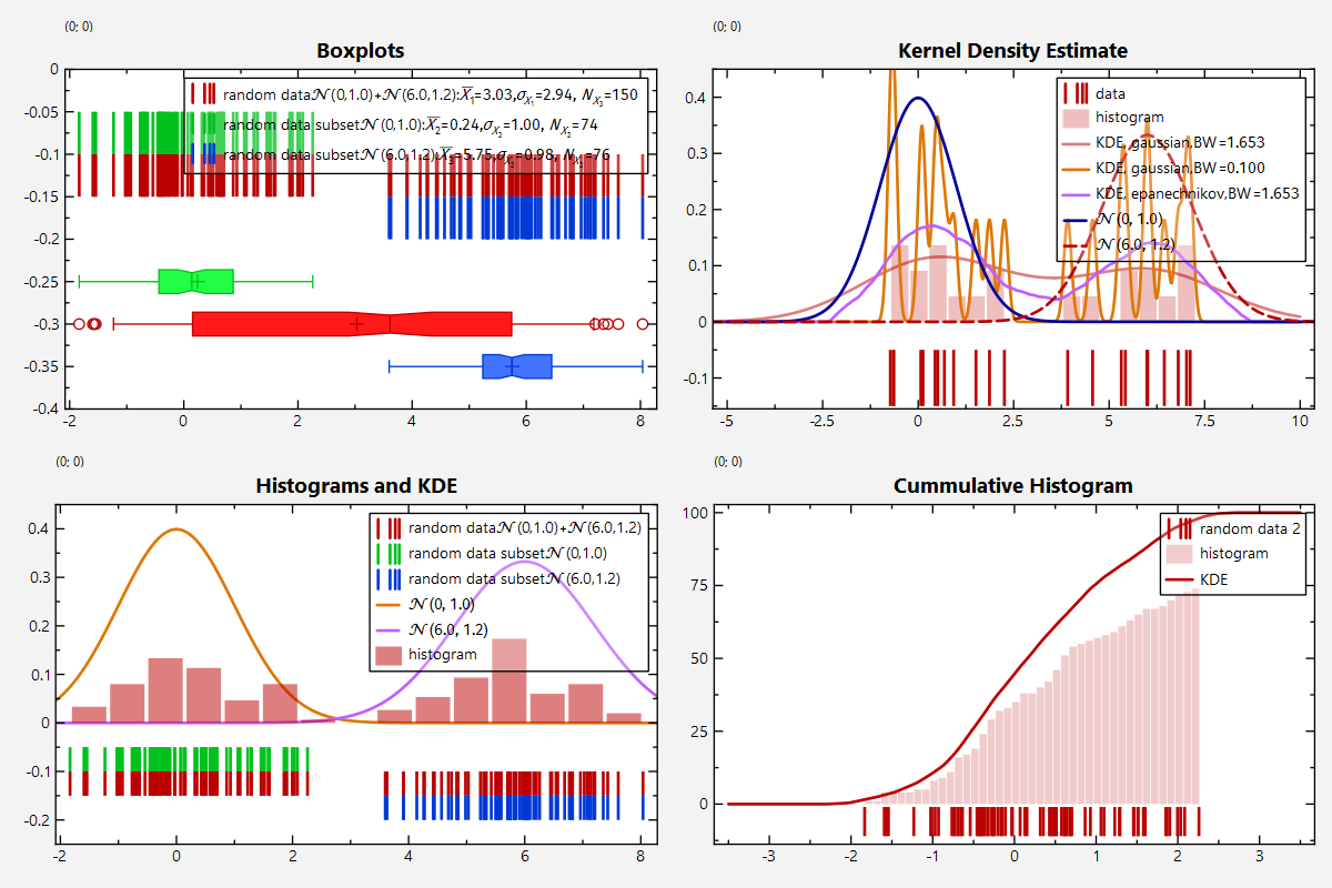
The output of the full test program [`datastore_statistics.cpp`](https://github.com/jkriege2/JKQtPlotter/tree/master/examples/datastore_statistics/datastore_statistics.cpp) looks like this:
|
|
|
|
|
|
|
|
|