mirror of
https://github.com/jkriege2/JKQtPlotter.git
synced 2024-11-16 02:25:50 +08:00
60 lines
2.9 KiB
Markdown
60 lines
2.9 KiB
Markdown
# Example (JKQTPlotter): Plotting Parametric Curves {#JKQTPlotterParametricCurves}
|
|
This project (see `./examples/parametriccurve/`) demonstrates how to draw parametric curves `[x,y]=f(t)`, using `JKQTPXYLineGraph` and `JKQTPXYParametrizedScatterGraph`, i.e. from a set of coordinates `[xi,yi]`, for which the vector-values function `f(t)` is evaluated explicitly. If you are alloking for an example of implicit drawing by only defining the function `f(t)` and having JKQTPlotter evaluate it automatically and adaptively, you'll have to use `JKQTPXYFunctionLineGraph`, which is explained in [`./examples/evalcurve`](https://github.com/jkriege2/JKQtPlotter/tree/master/examples/evalcurve)
|
|
|
|
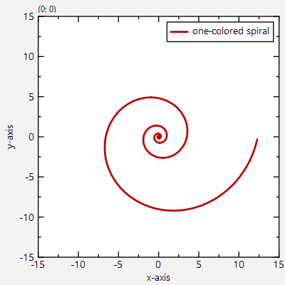
The source code of the main application can be found in [`parametriccurve.cpp`](https://github.com/jkriege2/JKQtPlotter/tree/master/examples/parametriccurve/parametriccurve.cpp). First, the parametric curve (here a [logarithic spiral](https://en.wikipedia.org/wiki/Logarithmic_spiral)) is sampled into two columns containing the x- and y-values along the curve. In addition the radial distance from x=y=0 is added into a third column:
|
|
```.cpp
|
|
QVector<double> X, Y, R;
|
|
const int Ndata=500; // number of plot points in each curve
|
|
const double phiMax=4.0*M_PI;
|
|
const double a=1;
|
|
const double k=0.2;
|
|
for (double phi=-phiMax; phi<=phiMax; phi+=phiMax/double(Ndata)) {
|
|
const double x=a*exp(k*phi)*cos(phi);
|
|
const double y=a*exp(k*phi)*sin(phi);
|
|
X<<x;
|
|
Y<<y;
|
|
R<<sqrt(x*x+y*y);
|
|
}
|
|
// and copy it to the datastore
|
|
size_t columnX=ds->addCopiedColumn(X, "x");
|
|
size_t columnY=ds->addCopiedColumn(Y, "y");
|
|
size_t columnR=ds->addCopiedColumn(R, "r");
|
|
```
|
|
|
|
|
|
Then simples graph just uses the columns X and Y to plot the curve:
|
|
```.cpp
|
|
JKQTPXYLineGraph* graph1=new JKQTPXYLineGraph(&plot);
|
|
graph1->setXColumn(columnX);
|
|
graph1->setYColumn(columnY);
|
|
graph1->setDrawLine(true);
|
|
graph1->setSymbolType(JKQTPNoSymbol);
|
|
graph1->setTitle("one-colored spiral");
|
|
plot.addGraph(graph1);
|
|
```
|
|
|
|
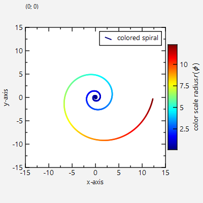
If you use `JKQTPXYParametrizedScatterGraph` instead of `JKQTPXYLineGraph`, you can also modify the color of the line-segments, connecting the datapoints:
|
|
```.cpp
|
|
JKQTPXYParametrizedScatterGraph* graph2=new JKQTPXYParametrizedScatterGraph(&plot2);
|
|
graph2->setXColumn(columnX);
|
|
graph2->setYColumn(columnY);
|
|
graph2->setColorColumn(columnR);
|
|
graph2->setColorPalette(ette(JKQTPMathImageMATLAB);
|
|
graph2->setSymbolType(JKQTPNoSymbol);
|
|
graph2->setDrawLine(true);
|
|
graph2->setTitle("colored spiral");
|
|
graph2->getColorBarRightAxis()->setAxisLabel("color scale radius $r(\\phi)$");
|
|
plot2.addGraph(graph2);
|
|
```
|
|
|
|
The result looks like this:
|
|
|
|

|
|
|
|
... and with the line-color set by the radius:
|
|
|
|

|
|
|
|
|
|
|