mirror of
https://github.com/jkriege2/JKQtPlotter.git
synced 2024-11-15 18:15:52 +08:00
124 lines
7.8 KiB
Markdown
124 lines
7.8 KiB
Markdown
# Example (JKQTPlotter): Violin Plots {#JKQTPlotterViolinplotGraphs}
|
|
|
|
[TOC]
|
|
[JKQTPlotterBasicJKQTPDatastoreStatistics]: @ref JKQTPlotterBasicJKQTPDatastoreStatistics "Advanced 1-Dimensional Statistics with JKQTPDatastore"
|
|
[statisticslibrary]: @ref jkqtptools_math_statistics "JKQTPlotter Statistics Library"
|
|
[JKQTPlotterBoxplotStyling]: @ref JKQTPlotterBoxplotStyling "Styling different aspects of boxplots"
|
|
|
|
This project (see [`violinplot`](https://github.com/jkriege2/JKQtPlotter/tree/master/examples/violinplot) demonstrates how to use JKQTPlotter to draw <a href="https://en.wikipedia.org/wiki/Violin_plot">violin plots</a> using the classes `JKQTPViolinplotVerticalElement` and `JKQTPViolinplotHorizontalElement`. Violin plots can be thought of as an extension to box plots, as they are also used to represent the distribution of a random variable, but contain more info than the "simple" 5-number statistics used for boxplots: Violin Plots show an estimate of the desnsity distribution of the random vriable, e.g. calculated as a kernel density estimate, or as a simple histogram. The Plotting classes themselves do not calculate these estimates, but only draw them into the plot. The density estimates are calculated by functions from the [statisticslibrary].
|
|
|
|
The source code of the main application is (see [`violinplot.cpp`](violinplot.cpp).
|
|
|
|
# Generating a test Dataset
|
|
|
|
First we generate some random numbers from a bimodal distribution (and as a by-product also from two single-distributions that form the bimodal):
|
|
```.cpp
|
|
size_t randomdatacol1=datastore1->addColumn("random data N(1,1)+N(6,2)");
|
|
size_t randomdatacol2=datastore1->addColumn("random data N(1,1)");
|
|
size_t randomdatacol3=datastore1->addColumn("random data N(6,2)");
|
|
std::random_device rd; // random number generators:
|
|
std::mt19937 gen{rd()};
|
|
std::uniform_int_distribution<> ddecide(0,1);
|
|
std::normal_distribution<> d1{1,1};
|
|
std::normal_distribution<> d2{6,2};
|
|
for (size_t i=0; i<50; i++) {
|
|
double v=0;
|
|
if (i%2==0) {
|
|
v=d1(gen);
|
|
datastore1->appendToColumn(randomdatacol2, v);
|
|
} else {
|
|
v=d2(gen);
|
|
datastore1->appendToColumn(randomdatacol3, v);
|
|
}
|
|
datastore1->appendToColumn(randomdatacol1, v);
|
|
}
|
|
```
|
|
|
|
# Visualizing data as a Rug Plot
|
|
|
|
Samples from the bimodal (built from two gaussian distributions `d1` and `d2`) are collected in `randomdatacol1`, whereas `randomdatacol2` and `randomdatacol3` collect those numbers that were drawn from `d1` or `d2` respectively.
|
|
|
|
Such data can be visualized by `JKQTPSingleColumnSymbolsGraph`, here using a rug plot (using `gData1->setPositionScatterStyle(JKQTPSingleColumnSymbolsGraph::RugPlot);` ... but also e.g. a ee swarm plot would be possible):
|
|
|
|
```.cpp
|
|
JKQTPSingleColumnSymbolsGraph* gData1;
|
|
plot->addGraph(gData1=new JKQTPSingleColumnSymbolsGraph(plot));
|
|
gData1->setPosition(0);
|
|
gData1->setPositionScatterStyle(JKQTPSingleColumnSymbolsGraph::RugPlot);
|
|
gData1->setDataColumn(randomdatacol1);
|
|
gData1->setDataDirection(JKQTPSingleColumnSymbolsGraph::DataDirection::Y);
|
|
```
|
|
|
|
# Drawing the (vertical) Violin Plot
|
|
|
|
Now we need to calculate the kernel density estimate from the data in `randomdatacol1` and store the result in two new columns `cViol1Cat` and `cViol1Freq`:
|
|
|
|
```.cpp
|
|
size_t cViol1Cat=datastore1->addColumn("violin 1, cat");
|
|
size_t cViol1Freq=datastore1->addColumn("violin 1, KDE");
|
|
jkqtpstatKDE1DAutoranged(datastore1->begin(randomdatacol1), datastore1->end(randomdatacol1),
|
|
datastore1->backInserter(cViol1Cat), datastore1->backInserter(cViol1Freq),
|
|
51, jkqtpstatKernel1DEpanechnikov,
|
|
jkqtpstatEstimateKDEBandwidth(datastore1->begin(randomdatacol1), datastore1->end(randomdatacol1)));
|
|
```
|
|
|
|
Finally we can add a `JKQTPViolinplotVerticalElement` to the plot and provide it with the kernel density estimate from above and with some additional statistical properties (minimum, maximum, average and median) of the dataset:
|
|
|
|
```.cpp
|
|
JKQTPViolinplotVerticalElement* gViol1;
|
|
plot->addGraph(gViol1=new JKQTPViolinplotVerticalElement(plot));
|
|
gViol1->setPos(2);
|
|
gViol1->setMin(jkqtpstatMinimum(datastore1->begin(randomdatacol1), datastore1->end(randomdatacol1)));
|
|
gViol1->setMax(jkqtpstatMaximum(datastore1->begin(randomdatacol1), datastore1->end(randomdatacol1)));
|
|
gViol1->setMean(jkqtpstatAverage(datastore1->begin(randomdatacol1), datastore1->end(randomdatacol1)));
|
|
gViol1->setMedian(jkqtpstatMedian(datastore1->begin(randomdatacol1), datastore1->end(randomdatacol1)));
|
|
gViol1->setViolinPositionColumn(cViol1Cat);
|
|
gViol1->setViolinFrequencyColumn(cViol1Freq);
|
|
gViol1->setColor(gData1->getSymbolColor());
|
|
gViol1->setViolinStyle(JKQTPGraphViolinplotStyleMixin::SmoothViolin);
|
|
gViol1->setViolinPositionMode(JKQTPGraphViolinplotStyleMixin::ViolinBoth);
|
|
```
|
|
|
|
The center of the `gData1` was set to 0 and the center of the violin plot is set to `2`. With `JKQTPViolinplotVerticalElement::setViolinStyle()` you can choose the style of the violin plot and with `JKQTPViolinplotVerticalElement::setViolinPositionMode()` you can select whether the density estimate should be displayed on the left, the right or on both sides of the center-line.
|
|
|
|
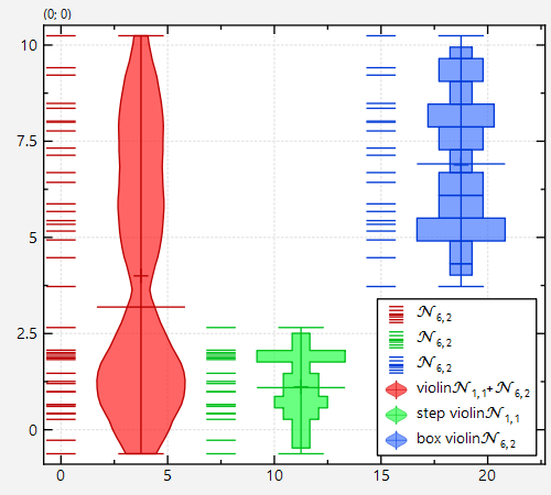
The result looks like this, if we use the same method as above to calculate also the violin plots for `randomdatacol2` and `randomdatacol3`:
|
|
|
|

|
|
|
|
Note that we set different styles for the three plots with:
|
|
```.cpp
|
|
gViol2->setViolinStyle(JKQTPGraphViolinplotStyleMixin::StepViolin); // green plot
|
|
gViol3->setViolinStyle(JKQTPGraphViolinplotStyleMixin::BoxViolin); // blue plot
|
|
```
|
|
|
|
Also for the green and blue plot, we did not calculate a kernel density estimate, but rather a simple histogram:
|
|
```.cpp
|
|
size_t cViol2Cat=datastore1->addColumn("violin 2, cat");
|
|
size_t cViol2Freq=datastore1->addColumn("violin 2, Histogram");
|
|
jkqtpstatHistogram1DAutoranged(datastore1->begin(randomdatacol2), datastore1->end(randomdatacol2),
|
|
datastore1->backInserter(cViol2Cat), datastore1->backInserter(cViol2Freq),
|
|
21, true, false, JKQTPStatHistogramBinXMode::XIsMid);
|
|
```
|
|
|
|
# Drawing a horizontal Violin Plot
|
|
|
|
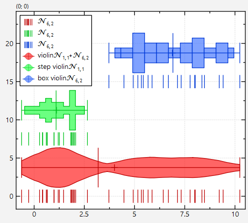
Finally note that if you use `JKQTPViolinplotHorizontalElement` instead of the `JKQTPViolinplotVerticalElement` used above, you can also draw horizontal violin plots:
|
|
|
|

|
|
|
|
|
|
# Adapters as shortcuts to drawing Violin Plots
|
|
|
|
Note that there also exist "adapters" that allow to draw violin plots in one line of code:
|
|
```.cpp
|
|
jkqtpstatAddVViolinplotHistogramAndOutliers(plot->getPlotter(), datastore1->begin(randomdatacol1), datastore1->end(randomdatacol1), -5);
|
|
jkqtpstatAddHViolinplotHistogramAndOutliers(plot->getPlotter(), datastore1->begin(randomdatacol1), datastore1->end(randomdatacol1), -5);
|
|
jkqtpstatAddVViolinplotHistogram(plot->getPlotter(), datastore1->begin(randomdatacol1), datastore1->end(randomdatacol1), -10);
|
|
jkqtpstatAddHViolinplotHistogram(plot->getPlotter(), datastore1->begin(randomdatacol1), datastore1->end(randomdatacol1), -10);
|
|
jkqtpstatAddVViolinplotKDEAndOutliers(plot->getPlotter(), datastore1->begin(randomdatacol1), datastore1->end(randomdatacol1), -15);
|
|
jkqtpstatAddHViolinplotKDEAndOutliers(plot->getPlotter(), datastore1->begin(randomdatacol1), datastore1->end(randomdatacol1), -15);
|
|
jkqtpstatAddVViolinplotKDE(plot->getPlotter(), datastore1->begin(randomdatacol1), datastore1->end(randomdatacol1), -20);
|
|
jkqtpstatAddHViolinplotKDE(plot->getPlotter(), datastore1->begin(randomdatacol1), datastore1->end(randomdatacol1), -20);
|
|
```
|
|
|