NEW/BREAKING: refactor CMake-Code, so static/dynamic switch is done via <code>BUILD_SHARED_LIBS</code>, which retires <code>JKQtPlotter_BUILD_STATIC_LIBS</code>, <code>JKQtPlotter_BUILD_SHARED_LIBS</code> and removes the capability to build static and shared libraries in one location (fixes issue #104) NEW: prepareed library for CMake's <a href="https://cmake.org/cmake/help/latest/module/FetchContent.html">FetchContent</a>-API NEW: the different sub-libraries JKQTPlotter, JKQTFastPlotter (DEPRECATED), JKQTMath, JKQTMathText can be activated/deactivated with CMake options JKQtPlotter_BUILD_LIB_JKQTPLOTTER, JKQtPlotter_BUILD_LIB_JKQTFASTPLOTTER, JKQtPlotter_BUILD_LIB_JKQTMATHTEXT, JKQtPlotter_BUILD_LIB_JKQTMATH |
||
|---|---|---|
| .. | ||
| CMakeLists.txt | ||
| README.md | ||
| violinplot_and_lib.pro | ||
| violinplot.cpp | ||
| violinplot.pro | ||
Example (JKQTPlotter): Violin Plots
[TOC] [JKQTPlotterBasicJKQTPDatastoreStatistics]: @ref JKQTPlotterBasicJKQTPDatastoreStatistics "Advanced 1-Dimensional Statistics with JKQTPDatastore" [statisticslibrary]: @ref jkqtptools_math_statistics "JKQTPlotter Statistics Library" [JKQTPlotterBoxplotStyling]: @ref JKQTPlotterBoxplotStyling "Styling different aspects of boxplots"
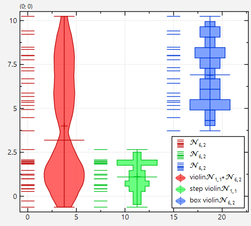
This project (see violinplot demonstrates how to use JKQTPlotter to draw violin plots using the classes JKQTPViolinplotVerticalElement and JKQTPViolinplotHorizontalElement. Violin plots can be thought of as an extension to box plots, as they are also used to represent the distribution of a random variable, but contain more info than the "simple" 5-number statistics used for boxplots: Violin Plots show an estimate of the desnsity distribution of the random vriable, e.g. calculated as a kernel density estimate, or as a simple histogram. The Plotting classes themselves do not calculate these estimates, but only draw them into the plot. The density estimates are calculated by functions from the [statisticslibrary].
The source code of the main application is (see violinplot.cpp.
Generating a test Dataset
First we generate some random numbers from a bimodal distribution (and as a by-product also from two single-distributions that form the bimodal):
    size_t randomdatacol1=datastore1->addColumn("random data N(1,1)+N(6,2)");
    size_t randomdatacol2=datastore1->addColumn("random data N(1,1)");
    size_t randomdatacol3=datastore1->addColumn("random data N(6,2)");
    std::random_device rd; // random number generators:
    std::mt19937 gen{rd()};
    std::uniform_int_distribution<> ddecide(0,1);
    std::normal_distribution<> d1{1,1};
    std::normal_distribution<> d2{6,2};
    for (size_t i=0; i<50; i++) {
        double v=0;
        if (i%2==0) {
            v=d1(gen);
            datastore1->appendToColumn(randomdatacol2, v);
        } else {
            v=d2(gen);
            datastore1->appendToColumn(randomdatacol3, v);
        }
        datastore1->appendToColumn(randomdatacol1, v);
    }
Visualizing data as a Rug Plot
Samples from the bimodal (built from two gaussian distributions d1 and d2) are collected in randomdatacol1, whereas randomdatacol2 and randomdatacol3 collect those numbers that were drawn from d1 or d2 respectively.
Such data can be visualized by JKQTPSingleColumnSymbolsGraph, here using a rug plot (using gData1->setPositionScatterStyle(JKQTPSingleColumnSymbolsGraph::RugPlot); ... but also e.g. a ee swarm plot would be possible):
    JKQTPSingleColumnSymbolsGraph* gData1;
    plot->addGraph(gData1=new JKQTPSingleColumnSymbolsGraph(plot));
    gData1->setPosition(0);
    gData1->setPositionScatterStyle(JKQTPSingleColumnSymbolsGraph::RugPlot);
    gData1->setDataColumn(randomdatacol1);
    gData1->setDataDirection(JKQTPSingleColumnSymbolsGraph::DataDirection::Y);
Drawing the (vertical) Violin Plot
Now we need to calculate the kernel density estimate from the data in randomdatacol1 and store the result in two new columns cViol1Cat and cViol1Freq:
    size_t cViol1Cat=datastore1->addColumn("violin 1, cat");
    size_t cViol1Freq=datastore1->addColumn("violin 1, KDE");
    jkqtpstatKDE1DAutoranged(datastore1->begin(randomdatacol1), datastore1->end(randomdatacol1),
                             datastore1->backInserter(cViol1Cat), datastore1->backInserter(cViol1Freq),
                             51, jkqtpstatKernel1DEpanechnikov,
                             jkqtpstatEstimateKDEBandwidth(datastore1->begin(randomdatacol1), datastore1->end(randomdatacol1)));
Finally we can add a JKQTPViolinplotVerticalElement to the plot and provide it with the kernel density estimate from above and with some additional statistical properties (minimum, maximum, average and median) of the dataset:
    JKQTPViolinplotVerticalElement* gViol1;
    plot->addGraph(gViol1=new JKQTPViolinplotVerticalElement(plot));
    gViol1->setPos(2);
    gViol1->setMin(jkqtpstatMinimum(datastore1->begin(randomdatacol1), datastore1->end(randomdatacol1)));
    gViol1->setMax(jkqtpstatMaximum(datastore1->begin(randomdatacol1), datastore1->end(randomdatacol1)));
    gViol1->setMean(jkqtpstatAverage(datastore1->begin(randomdatacol1), datastore1->end(randomdatacol1)));
    gViol1->setMedian(jkqtpstatMedian(datastore1->begin(randomdatacol1), datastore1->end(randomdatacol1)));
    gViol1->setViolinPositionColumn(cViol1Cat);
    gViol1->setViolinFrequencyColumn(cViol1Freq);
    gViol1->setColor(gData1->getSymbolColor());
    gViol1->setViolinStyle(JKQTPGraphViolinplotStyleMixin::SmoothViolin);
    gViol1->setViolinPositionMode(JKQTPGraphViolinplotStyleMixin::ViolinBoth);
The center of the gData1 was set to 0 and the center of the violin plot is set to 2. With JKQTPViolinplotVerticalElement::setViolinStyle() you can choose the style of the violin plot and with JKQTPViolinplotVerticalElement::setViolinPositionMode() you can select whether the density estimate should be displayed on the left, the right or on both sides of the center-line.
The result looks like this, if we use the same method as above to calculate also the violin plots for randomdatacol2 and randomdatacol3:
Note that we set different styles for the three plots with:
    gViol2->setViolinStyle(JKQTPGraphViolinplotStyleMixin::StepViolin); // green plot
    gViol3->setViolinStyle(JKQTPGraphViolinplotStyleMixin::BoxViolin);  // blue plot
Also for the green and blue plot, we did not calculate a kernel density estimate, but rather a simple histogram:
    size_t cViol2Cat=datastore1->addColumn("violin 2, cat");
    size_t cViol2Freq=datastore1->addColumn("violin 2, Histogram");
    jkqtpstatHistogram1DAutoranged(datastore1->begin(randomdatacol2), datastore1->end(randomdatacol2),
                             datastore1->backInserter(cViol2Cat), datastore1->backInserter(cViol2Freq),
                             21, true, false, JKQTPStatHistogramBinXMode::XIsMid);
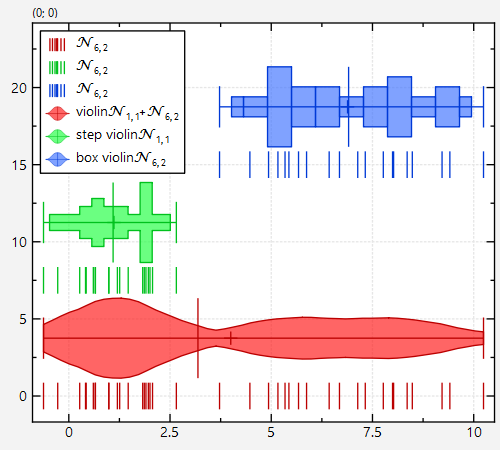
Drawing a horizontal Violin Plot
Finally note that if you use JKQTPViolinplotHorizontalElement instead of the JKQTPViolinplotVerticalElement used above, you can also draw horizontal violin plots:
Adapters as shortcuts to drawing Violin Plots
Note that there also exist "adapters" that allow to draw violin plots in one line of code:
    jkqtpstatAddVViolinplotHistogramAndOutliers(plot->getPlotter(), datastore1->begin(randomdatacol1), datastore1->end(randomdatacol1), -5);
    jkqtpstatAddHViolinplotHistogramAndOutliers(plot->getPlotter(), datastore1->begin(randomdatacol1), datastore1->end(randomdatacol1), -5);
    jkqtpstatAddVViolinplotHistogram(plot->getPlotter(), datastore1->begin(randomdatacol1), datastore1->end(randomdatacol1), -10);
    jkqtpstatAddHViolinplotHistogram(plot->getPlotter(), datastore1->begin(randomdatacol1), datastore1->end(randomdatacol1), -10);
    jkqtpstatAddVViolinplotKDEAndOutliers(plot->getPlotter(), datastore1->begin(randomdatacol1), datastore1->end(randomdatacol1), -15);
    jkqtpstatAddHViolinplotKDEAndOutliers(plot->getPlotter(), datastore1->begin(randomdatacol1), datastore1->end(randomdatacol1), -15);
    jkqtpstatAddVViolinplotKDE(plot->getPlotter(), datastore1->begin(randomdatacol1), datastore1->end(randomdatacol1), -20);
    jkqtpstatAddHViolinplotKDE(plot->getPlotter(), datastore1->begin(randomdatacol1), datastore1->end(randomdatacol1), -20);

