| .. | ||
| CMakeLists.txt | ||
| contourplot_and_lib.pro | ||
| contourplot.cpp | ||
| contourplot.pro | ||
| contourplotanimator.cpp | ||
| contourplotanimator.h | ||
| README.md | ||
Example (JKQTPlotter): Contour Plots
This project (see ./examples/contourplot/) shows how to draw contour plots with JKQTPlotter.
[TOC]
Drawing a Contour Plot
The source code of the main application is (see contourplot.cpp ).
First the electric potential from a quadrupole is calculated and stored in an image column inside the JKQTPDatastore:
    JKQTPDatastore* ds=plot.getDatastore();

    const int NX=500; // image dimension in x-direction [pixels]
    const int NY=500; // image dimension in y-direction [pixels]
    const double w=2.7e-6;
    const double dx=w/static_cast<double>(NX);
    const double h=NY*dx;
    size_t cPotential=ds->addImageColumn(NX, NY, "imagedata");

    double x;
    double y=-h/2.0;
    const double eps0=8.854187e-12;
    const double Q1=1.6e-19;           // charge of charged particle 1
    const double Q1_x0=-0.5e-6;        // x-position of charged particle 1
    const double Q1_y0=-0.5e-6;        // y-position of charged particle 1
    const double Q2=1.6e-19;           // charge of charged particle 2
    const double Q2_x0=0.5e-6;         // x-position of charged particle 2
    const double Q2_y0=0.5e-6;         // y-position of charged particle 2
    const double Q3=-1.6e-19;          // charge of charged particle 3
    const double Q3_x0=-0.5e-6;        // x-position of charged particle 3
    const double Q3_y0=0.5e-6;         // y-position of charged particle 3
    const double Q4=-1.6e-19;          // charge of charged particle 4
    const double Q4_x0=0.5e-6;         // x-position of charged particle 4
    const double Q4_y0=-0.5e-6;        // y-position of charged particle 4
    for (size_t iy=0; iy<NY; iy++ ) {
        x=-w/2.0;
        for (size_t ix=0; ix<NX; ix++ ) {
            const double r1=sqrt((x-Q1_x0)*(x-Q1_x0)+(y-Q1_y0)*(y-Q1_y0));
            const double r2=sqrt((x-Q2_x0)*(x-Q2_x0)+(y-Q2_y0)*(y-Q2_y0));
            const double r3=sqrt((x-Q3_x0)*(x-Q3_x0)+(y-Q3_y0)*(y-Q3_y0));
            const double r4=sqrt((x-Q4_x0)*(x-Q4_x0)+(y-Q4_y0)*(y-Q4_y0));
            ds->setPixel(cPotential, ix, iy, Q1/(4.0*M_PI*eps0)/r1+Q2/(4.0*M_PI*eps0)/r2+Q3/(4.0*M_PI*eps0)/r3+Q4/(4.0*M_PI*eps0)/r4);
            x+=dx;
        }
        y+=dx;
    }
Then this image column can be drawn with a JKQTPColumnContourPlot:
    JKQTPColumnContourPlot* graph=new JKQTPColumnContourPlot(&plot);
    graph->setTitle("");
    // image column with the data
    graph->setImageColumn(cPotential);
    // where does the image start in the plot, given in plot-axis-coordinates (bottom-left corner)
    graph->setX(-w/2.0);
    graph->setY(-h/2.0);
    // width and height of the image in plot-axis-coordinates
    graph->setWidth(w);
    graph->setHeight(h);
    // color-map is "BlueGreenRed"
    graph->setPalette(JKQTPMathImageBlueGreenRed);
    // get coordinate axis of color-bar and set its label
    graph->getColorBarRightAxis()->setAxisLabel("electric potential [V]");
    // add some levels for the contours. These are chosen to be at the actual potential values
    // at several specified relative distance from Q1, i.e. at phi(Q1_x0*reldist) (phi: potential of Q1)
    QVector<double> reldists; reldists<<0.1<<0.25<<0.5<<1<<1.5<<2<<2.5<<3;
    // finally contour levels with +1 and -1 sign are added to show the positive and negative potential:
    for (auto reldist: reldists) {
        const double level=fabs(Q1/(4.0*M_PI*eps0)/(Q1_x0*reldist));
        graph->addContourLevel(-level);
        graph->addContourLevel(level);
    }
    qDebug()<<graph->getContourLevels();
    graph->setAutoImageRange(false);
    graph->setImageMin(graph->getContourLevels().first());
    graph->setImageMax(graph->getContourLevels().last());
Note that we created the list of contour levels to draw explicitly here using JKQTPColumnContourPlot::addContourLevel(). There are also methods JKQTPColumnContourPlot::createContourLevels() and JKQTPColumnContourPlot::createContourLevelsLog() to auto-generate these from the data-range with linear or logarithmic spacing, but both options do not yield good results here. The code above generates these contour levels:
-0.0287602, -0.0115041, -0.00575203, -0.00287602, -0.00191734, -0.00143801, -0.00115041, -0.000958672, 0.000958672, 0.00115041, 0.00143801, 0.00191734, 0.00287602, 0.00575203, 0.0115041, 0.0287602
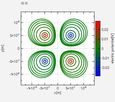
The result looks like this:
Styling a Contour Plot
You can change the way that the colors for the contours are chosen by calling JKQTPColumnContourPlot::setContourColoringMode() with another mode:
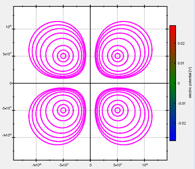
JKQTPColumnContourPlot::SingleColorContoursuses the same color (set byJKQTPColumnContourPlot::setLineColor()) for all contours.
JKQTPColumnContourPlot::ColorContoursFromPaletteByValueis the mode used for the example above, which chooses the color from the current color-palette based on the current image data range and the actual level of the contour line.
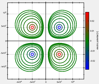
JKQTPColumnContourPlot::ColorContoursFromPalettechooses the color by evenly spacing the contour lines over the full color palette. the line-color will then have no connection to the actual value of the level.
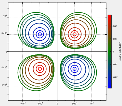
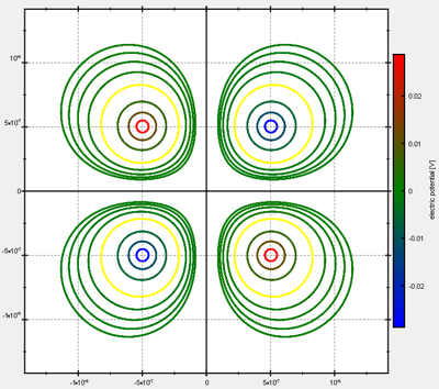
In all modes you can override the coloring of single levels by calling JKQTPColumnContourPlot::setOverrideColor(level, color). In the example above this looks like this:
    for (auto reldist: reldists) {
        const double level=fabs(Q1/(4.0*M_PI*eps0)/(Q1_x0*reldist));
        graph->addContourLevel(-level);
        graph->addContourLevel(level);

        // set a special color for some lines:
        if (reldist==1) {
            graph->setOverrideColor(-level, QColor("yellow"));
            graph->setOverrideColor(level, QColor("yellow"));
        }
    }
This code results (in the default coloring mode JKQTPColumnContourPlot::ColorContoursFromPaletteByValue) in:
Gimmick: Animating a Contour Plot
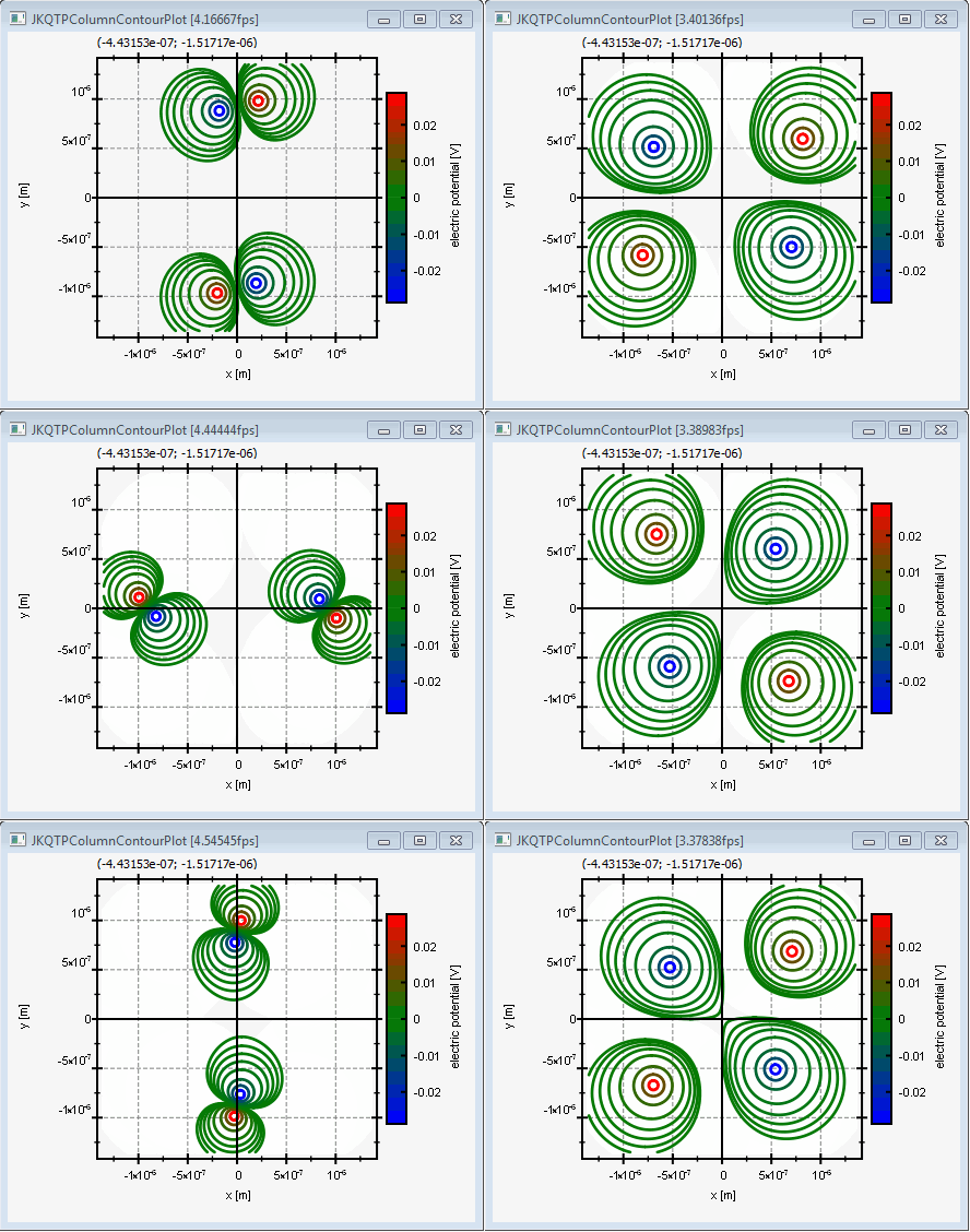
In order to demonstrate the caching implemented in the contour plot, there is optional animation code inside this example, in the form of the class ContourPlotAnimator (see (see ContourPlotAnimator.cpp ).
The code therein results in an animation like this:
Note that zooming can still be perfomred without the need to recalculate the contour lines.
