# Example (JKQTPlotter): Contour Plots {#JKQTPlotterContourPlot}
This project (see `./examples/contourplot/`) shows how to draw contour plots with JKQTPlotter.
[TOC]
# Drawing a Contour Plot
The source code of the main application is (see [`contourplot.cpp`](https://github.com/jkriege2/JKQtPlotter/tree/master/examples/contourplot/contourplot.cpp) ).
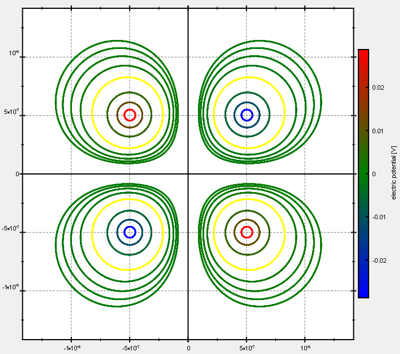
First the electric potential from a quadrupole is calculated and stored in an image column inside the JKQTPDatastore:
```.cpp
JKQTPDatastore* ds=plot.getDatastore();
const int NX=500; // image dimension in x-direction [pixels]
const int NY=500; // image dimension in y-direction [pixels]
const double w=2.7e-6;
const double dx=w/static_cast<double>(NX);
const double h=NY*dx;
size_t cPotential=ds->addImageColumn(NX, NY, "imagedata");
double x;
double y=-h/2.0;
const double eps0=8.854187e-12;
const double Q1=1.6e-19; // charge of charged particle 1
const double Q1_x0=-0.5e-6; // x-position of charged particle 1
const double Q1_y0=-0.5e-6; // y-position of charged particle 1
const double Q2=1.6e-19; // charge of charged particle 2
const double Q2_x0=0.5e-6; // x-position of charged particle 2
const double Q2_y0=0.5e-6; // y-position of charged particle 2
const double Q3=-1.6e-19; // charge of charged particle 3
const double Q3_x0=-0.5e-6; // x-position of charged particle 3
const double Q3_y0=0.5e-6; // y-position of charged particle 3
const double Q4=-1.6e-19; // charge of charged particle 4
const double Q4_x0=0.5e-6; // x-position of charged particle 4
const double Q4_y0=-0.5e-6; // y-position of charged particle 4
for (size_t iy=0; iy<NY; iy++ ) {
x=-w/2.0;
for (size_t ix=0; ix<NX; ix++ ) {
const double r1=sqrt((x-Q1_x0)*(x-Q1_x0)+(y-Q1_y0)*(y-Q1_y0));
const double r2=sqrt((x-Q2_x0)*(x-Q2_x0)+(y-Q2_y0)*(y-Q2_y0));
const double r3=sqrt((x-Q3_x0)*(x-Q3_x0)+(y-Q3_y0)*(y-Q3_y0));
const double r4=sqrt((x-Q4_x0)*(x-Q4_x0)+(y-Q4_y0)*(y-Q4_y0));
ds->setPixel(cPotential, ix, iy, Q1/(4.0*M_PI*eps0)/r1+Q2/(4.0*M_PI*eps0)/r2+Q3/(4.0*M_PI*eps0)/r3+Q4/(4.0*M_PI*eps0)/r4);
x+=dx;
}
y+=dx;
}
```
Then this image column can be drawn with a `JKQTPColumnContourPlot`:
```.cpp
JKQTPColumnContourPlot* graph=new JKQTPColumnContourPlot(&plot);
graph->setTitle("");
// image column with the data
graph->setImageColumn(cPotential);
// where does the image start in the plot, given in plot-axis-coordinates (bottom-left corner)
graph->setX(-w/2.0);
graph->setY(-h/2.0);
// width and height of the image in plot-axis-coordinates
graph->setWidth(w);
graph->setHeight(h);
// color-map is "BlueGreenRed"
graph->setColorPalette(JKQTPMathImageBlueGreenRed);
// get coordinate axis of color-bar and set its label
graph->getColorBarRightAxis()->setAxisLabel("electric potential [V]");
// add some levels for the contours. These are chosen to be at the actual potential values
// at several specified relative distance from Q1, i.e. at phi(Q1_x0*reldist) (phi: potential of Q1)
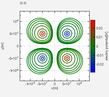
QVector<double> reldists; reldists<<0.1<<0.25<<0.5<<1<<1.5<<2<<2.5<<3;
// finally contour levels with +1 and -1 sign are added to show the positive and negative potential:
for (auto reldist: reldists) {
const double level=fabs(Q1/(4.0*M_PI*eps0)/(Q1_x0*reldist));
graph->addContourLevel(-level);
graph->addContourLevel(level);
}
qDebug()<<graph->getContourLevels();
graph->setAutoImageRange(false);
graph->setImageMin(graph->getContourLevels().first());
graph->setImageMax(graph->getContourLevels().last());
```
Note that we created the list of contour levels to draw explicitly here using `JKQTPColumnContourPlot::addContourLevel()`. There are also methods `JKQTPColumnContourPlot::createContourLevels()` and `JKQTPColumnContourPlot::createContourLevelsLog()` to auto-generate these from the data-range with linear or logarithmic spacing, but both options do not yield good results here. The code above generates these contour levels:
```
-0.0287602, -0.0115041, -0.00575203, -0.00287602, -0.00191734, -0.00143801, -0.00115041, -0.000958672, 0.000958672, 0.00115041, 0.00143801, 0.00191734, 0.00287602, 0.00575203, 0.0115041, 0.0287602
```
The result looks like this:
# Styling a Contour Plot
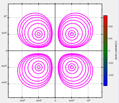
You can change the way that the colors for the contours are chosen by calling `JKQTPColumnContourPlot::setContourColoringMode()` with another mode:
- `JKQTPColumnContourPlot::SingleColorContours` uses the same color (set by `JKQTPColumnContourPlot::setLineColor()`) for all contours.<br>
- `JKQTPColumnContourPlot::ColorContoursFromPaletteByValue` is the mode used for the example above, which chooses the color from the current color-palette based on the current image data range and the actual level of the contour line. <br>
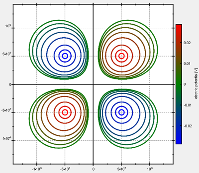
- `JKQTPColumnContourPlot::ColorContoursFromPalette` chooses the color by evenly spacing the contour lines over the full color palette. the line-color will then have no connection to the actual value of the level.<br>
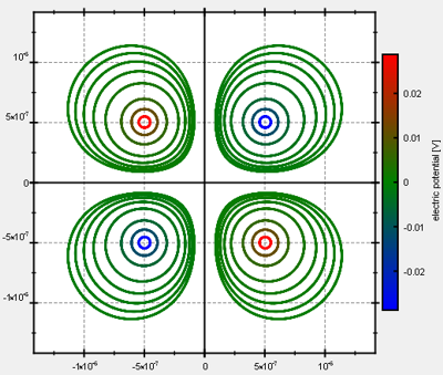
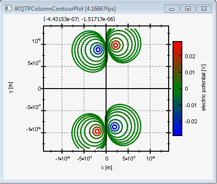
In all modes you can override the coloring of single levels by calling `JKQTPColumnContourPlot::setOverrideColor(level, color)`. In the example above this looks like this:
```.cpp
for (auto reldist: reldists) {
const double level=fabs(Q1/(4.0*M_PI*eps0)/(Q1_x0*reldist));
graph->addContourLevel(-level);
graph->addContourLevel(level);
// set a special color for some lines:
if (reldist==1) {
graph->setOverrideColor(-level, QColor("yellow"));
graph->setOverrideColor(level, QColor("yellow"));
}
}
```
This code results (in the default coloring mode `JKQTPColumnContourPlot::ColorContoursFromPaletteByValue`) in:
# Gimmick: Animating a Contour Plot
In order to demonstrate the caching implemented in the contour plot, there is optional animation code inside this example, in the form of the class `ContourPlotAnimator` (see (see [`ContourPlotAnimator.cpp`](https://github.com/jkriege2/JKQtPlotter/tree/master/examples/contourplot/ContourPlotAnimator.cpp) ).
The code therein results in an animation like this:
Note that zooming can still be perfomred without the need to recalculate the contour lines.